MatPlotLib is innate Python
Table of Contents
GNU Octave meets Python
Data importing
import numpy as np
import scipy.io


def read_dataset(filename):
    """Reads data from .mat binary file."""
    data = scipy.io.loadmat(filename)
    return [data[k] for k in ('neg_examples_nobias',
                              'pos_examples_nobias',
                              'w_init', 'w_gen_feas')]
(nen, pen, wi, wg) = read_dataset('data/dataset1.mat')
print(nen, '\n\n', pen, '\n\n', wi, '\n\n', wg)
print(type(nen))
[[-0.80857143  0.8372093 ]
 [ 0.35714286  0.85049834]
 [-0.75142857 -0.73089701]
 [-0.3         0.12624585]]

 [[ 0.87142857  0.62458472]
 [-0.02       -0.92358804]
 [ 0.36285714 -0.31893688]
 [ 0.88857143 -0.87043189]]

 [[-0.62170147]
 [ 0.76091527]
 [ 0.77187205]]

 [[ 4.3496526 ]
 [-2.60997235]
 [-0.69414749]]
<class 'numpy.ndarray'>
NdArray manipulations
Directly
for i in nen:
    print(i[0], i[1], type(i[1]), '\n')
... -0.808571428571 0.837209302326 <class 'numpy.float64'>

0.357142857143 0.85049833887 <class 'numpy.float64'>

-0.751428571429 -0.730897009967 <class 'numpy.float64'>

-0.3 0.126245847176 <class 'numpy.float64'>
Converted
for i in nen.tolist():
    print(i[0], i[1], type(i[1]), '\n')
... -0.8085714285714286 0.8372093023255818 <class 'float'>

0.3571428571428572 0.8504983388704321 <class 'float'>

-0.7514285714285714 -0.7308970099667773 <class 'float'>

-0.2999999999999999 0.1262458471760799 <class 'float'>
Data visualization
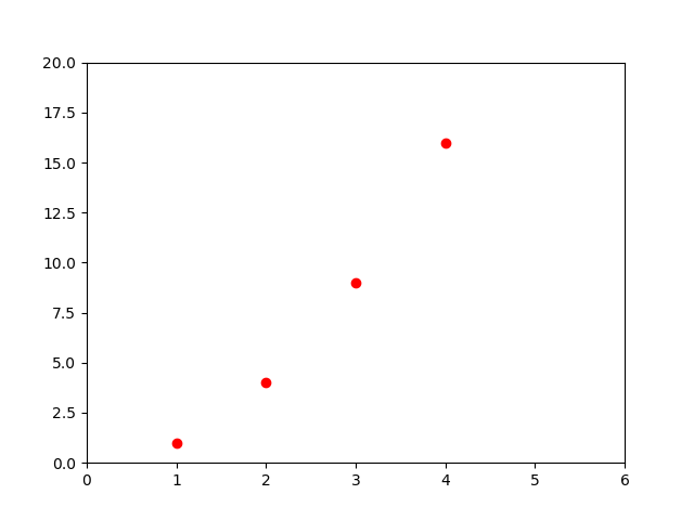
Simple
import matplotlib.pyplot as plt
plt.plot([1,2,3,4], [1,4,9,16], 'ro')
plt.axis([0, 6, 0, 20])
plt.savefig('img/plt/first_test.png')
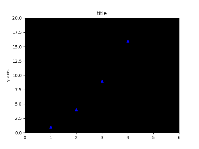
Colorization
ax = plt.gca()
ax.set_axis_bgcolor('black')
# ax.set_axis_bgcolor((1, 0, 0))
plt.plot([1,2,3,4], [1,4,9,16], 'b^')
plt.axis([0, 6, 0, 20])
plt.savefig('img/plt/second_test.png')
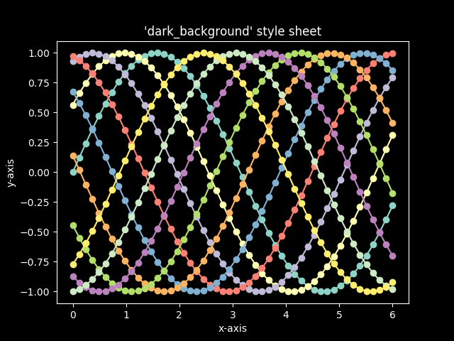
Full-fledged dark theme
import numpy as np
import matplotlib.pyplot as plt


plt.style.use('dark_background')

fig, ax = plt.subplots()

L = 6
x = np.linspace(0, L)
ncolors = len(plt.rcParams['axes.prop_cycle'])
shift = np.linspace(0, L, ncolors, endpoint=False)
for s in shift:
    ax.plot(x, np.sin(x + s), 'o-')
ax.set_xlabel('x-axis')
ax.set_ylabel('y-axis')
ax.set_title("'dark_background' style sheet")

plt.savefig('img/plt/dark_test.png')
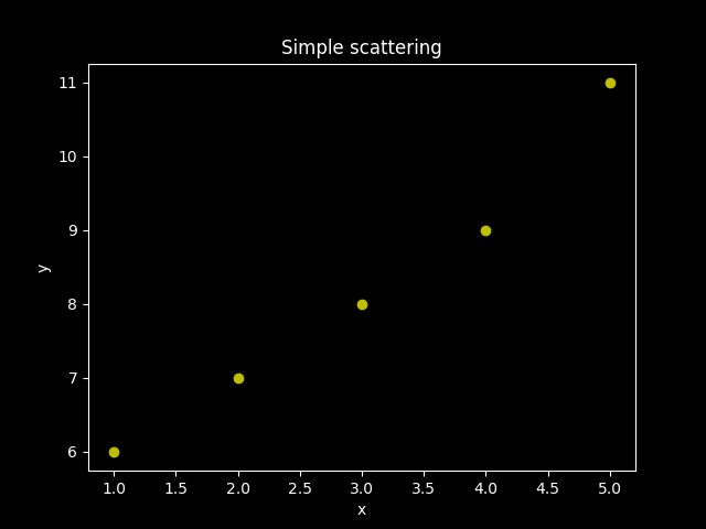
Scattering
import matplotlib.pyplot as plt

plt.style.use('dark_background')

x = [1, 2, 3, 4, 5]
y = [6, 7, 8, 9, 11]

plt.scatter(x, y, color='y')

plt.xlabel('x')
plt.ylabel('y')
plt.title('Simple scattering')
plt.savefig('img/plt/simple_scatter.png')
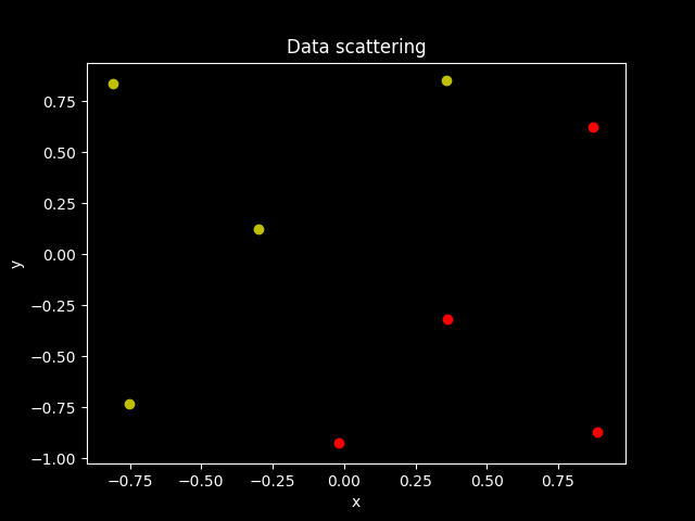
All together
import matplotlib.pyplot as plt

plt.style.use('dark_background')
data_neg = [[-0.80857143, 0.8372093],
            [ 0.35714286, 0.85049834],
            [-0.75142857, -0.73089701],
            [-0.3, 0.12624585]]

data_pos = [[0.87142857, 0.62458472],
            [-0.02, -0.92358804],
            [0.36285714, -0.31893688],
            [ 0.88857143, -0.87043189]]

for i in data_neg:
    plt.scatter(i[0], i[1], color='y')

for i in data_pos:
    plt.scatter(i[0], i[1], color='r')


plt.xlabel('x')
plt.ylabel('y')
plt.title('Data scattering')
plt.savefig('img/plt/data_scatter.png')
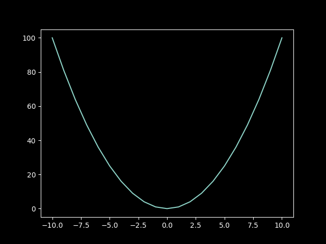
Parabola
import numpy as np
from math import exp
import matplotlib.pyplot as plt


def custom_function(x):  # sigmoid(x):
    return x * x  # 1. / (1 + exp(-x))


x = np.array(range(-10, 11))
y = custom_function(x)  #sigmoid(x)
plt.style.use('dark_background')
plt.plot(x, y)
plt.savefig('img/plt/sigmoidal_f.png')
Four datasets on one picture
Iterate the dataset
datasets = ['data/dataset1.mat', 'data/dataset2.mat',
            'data/dataset3.mat', 'data/dataset4.mat']
for i in datasets:
    (nen, pen, wi, wg) = read_dataset(i)
    print(nen, '\n\n', pen, '\n\n', wi, '\n\n', wg)
    print('\n\n\n')
>>> ... ... ... ... [[-0.80857143  0.8372093 ]
 [ 0.35714286  0.85049834]
 [-0.75142857 -0.73089701]
 [-0.3         0.12624585]]

 [[ 0.87142857  0.62458472]
 [-0.02       -0.92358804]
 [ 0.36285714 -0.31893688]
 [ 0.88857143 -0.87043189]]

 [[-0.62170147]
 [ 0.76091527]
 [ 0.77187205]]

 [[ 4.3496526 ]
 [-2.60997235]
 [-0.69414749]]


[[-0.80857143  0.8372093 ]
 [ 0.35714286  0.85049834]
 [-0.75142857 -0.73089701]
 [-0.3         0.12624585]
 [ 0.64285714 -0.5448505 ]]

 [[ 0.87142857  0.62458472]
 [-0.02       -0.92358804]
 [ 0.36285714 -0.31893688]
 [ 0.88857143 -0.87043189]
 [-0.52857143  0.51162791]]

 [[ 1.84689887]
 [-0.58324929]
 [-0.54178883]]

 []


[[-0.79142857  0.07973422]
 [-0.55714286  0.41196013]
 [-0.22571429  0.69767442]
 [ 0.16285714  0.83056478]
 [ 0.46        0.65780731]
 [ 0.73428571  0.33887043]
 [ 0.82571429 -0.01328904]]

 [[-0.76285714 -0.19269103]
 [-0.60285714 -0.48504983]
 [-0.38571429 -0.69767442]
 [-0.19142857 -0.35880399]
 [ 0.28285714 -0.43189369]
 [ 0.40857143 -0.69767442]
 [ 0.75142857 -0.23255814]]

 [[ 0.90368034]
 [-0.49087549]
 [ 0.94855295]]

 [[ -0.67272864]
 [-11.48921717]
 [ -0.89411095]]


[[-0.86571429 -0.39202658]
 [-0.78571429 -0.17275748]
 [-0.55714286  0.24584718]
 [-0.28857143  0.52491694]
 [-0.12857143  0.52491694]
 [ 0.08285714  0.33222591]
 [ 0.18        0.10631229]
 [ 0.25428571 -0.16611296]
 [ 0.32857143 -0.35215947]]

 [[-0.08857143  0.23255814]
 [ 0.00857143 -0.06644518]
 [ 0.12857143 -0.3255814 ]
 [ 0.28857143 -0.52491694]
 [ 0.59714286 -0.46511628]
 [ 0.71714286 -0.1461794 ]
 [ 0.86        0.15946844]
 [ 0.94571429  0.44518272]]

 [[-0.03182596]
 [-0.25511273]
 [-0.00710252]]

 []
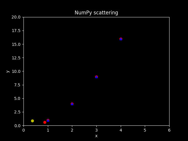
Scatter NumPy array
import matplotlib.pyplot as plt

plt.style.use('dark_background')
(data_neg, data_pos, wi, wg) = read_dataset('data/dataset1.mat')

for i in data_neg:
    plt.scatter(i[0], i[1], color='y')

for i in data_pos:
    plt.scatter(i[0], i[1], color='r')


plt.xlabel('x')
plt.ylabel('y')
plt.title('NumPy scattering')
plt.savefig('img/plt/ndarray_scatter.png')
Scatter several datasets on one image
import scipy.io
import matplotlib.pyplot as plt


def read_dataset(filename):
    """Reads data from .mat binary file."""
    data = scipy.io.loadmat(filename)
    return [data[k] for k in ('neg_examples_nobias',
                              'pos_examples_nobias',
                              'w_init', 'w_gen_feas')]


datasets = ['data/dataset1.mat', 'data/dataset2.mat',
            'data/dataset3.mat', 'data/dataset4.mat']

plt.style.use('dark_background')
fig = plt.figure()

for i, data in enumerate(datasets):
    (data_neg, data_pos, wi, wg) = read_dataset(data)
    s1 = fig.add_subplot(2, 2, i+1)
    for i in data_neg:
        s1.scatter(i[0], i[1], color='y')
    for i in data_pos:
        s1.scatter(i[0], i[1], color='r')

plt.savefig('img/plt/four_datasets.png')

blog comments powered by Disqus